[1]:
import os

os.chdir("siesta_1")
import numpy as np
import sisl as si
from sisl.viz import merge_plots
from sisl.viz.processors.math import normalize
from functools import partial
import matplotlib.pyplot as plt

%matplotlib inline
Siesta — the H2O molecule
This tutorial will describe a complete walk-through of some of the sisl functionalities that may be related to the Siesta code.
Creating the geometry
Our system of interest will be the \(\mathrm H_2\mathrm O\) system. The first task will be to create the molecule geometry. This is done using lists of atomic coordinates and atomic species. Additionally one needs to define the lattice (or if you prefer: unit-cell) where the molecule resides in. Siesta is a periodic DFT code and thus all directions are periodic. I.e. when simulating molecules it is vital to have a large vacuum gap between periodic images. In this case we use a supercell of side-lengths \(10\mathrm{Ang}\).
[2]:
h2o = si.Geometry(
    [[0, 0, 0], [0.8, 0.6, 0], [-0.8, 0.6, 0.0]],
    [si.Atom("O"), si.Atom("H"), si.Atom("H")],
    lattice=si.Lattice(10, origin=[-5] * 3),
)
The input are the 1) xyz coordinates, 2) the atomic species and 3) the lattice that is attached.
By printing the object one gets basic information regarding the geometry, such as 1) number of atoms, 2) species of atoms, 3) number of orbitals, 4) orbitals associated with each atom and 5) number of supercells (should be 1 for molecules).
[3]:
print(h2o)
Geometry{na: 3, no: 3,
 Atoms{species: 2,
  Atom{O, Z: 8, mass(au): 15.99940, maxR: -1.00000,
   Orbital{R: -1.00000, q0: 0.0}
  }: 1,
  Atom{H, Z: 1, mass(au): 1.00794, maxR: -1.00000,
   Orbital{R: -1.00000, q0: 0.0}
  }: 2,
 },
 maxR: -1.00000,
 Lattice{nsc: [1 1 1],
  origin=[-5.0000, -5.0000, -5.0000],
  A=[10.0000, 0.0000, 0.0000],
  B=[0.0000, 10.0000, 0.0000],
  C=[0.0000, 0.0000, 10.0000],
  bc=[Periodic,
      Periodic,
      Periodic]
 }
}
Lets visualize the atomic positions (here adding atomic indices)
[4]:
h2o.plot(axes="xy")
Now we need to create the input fdf file for Siesta:
[5]:
open("RUN.fdf", "w").write(
    """%include STRUCT.fdf
SystemLabel siesta_1
PAO.BasisSize SZP
MeshCutoff 250. Ry
CDF.Save true
CDF.Compress 9
SaveHS true
SaveRho true
"""
)
h2o.write("STRUCT.fdf")
h2o) to write its information to the file STRUCT.fdf.LatticeConstantLatticeVectorsNumberOfAtomsAtomicCoordinatesFormatAtomicCoordinatesAndAtomicSpeciesNumberOfSpeciesChemicalSpeciesLabel
Creating the electronic structure
Before continuing we need to run Siesta to calculate the electronic structure.
siesta RUN.fdf
After having completed the Siesta run we may read the Siesta output to manipulate and extract different information.
[6]:
fdf = si.get_sile("RUN.fdf")
H = fdf.read_hamiltonian()
# Create a short-hand to handle the geometry
h2o = H.geometry
print(H)
Hamiltonian{non-zero: 289, orthogonal: False,
 Spin{unpolarized},
 Geometry{na: 3, no: 17,
  Atoms{species: 2,
   Atom{O, Z: 8, mass(au): 16.00000, maxR: 2.05640,
    AtomicOrbital{2sZ1, q0: 2.0, SphericalOrbital{l: 0, R: 1.7096999999999989, q0: 2.0}},
    AtomicOrbital{2pyZ1, q0: 1.3333333333333333, SphericalOrbital{l: 1, R: 2.036900000000015, q0: 4.0}},
    AtomicOrbital{2pzZ1, q0: 1.3333333333333333, SphericalOrbital{l: 1, R: 2.036900000000015, q0: 4.0}},
    AtomicOrbital{2pxZ1, q0: 1.3333333333333333, SphericalOrbital{l: 1, R: 2.036900000000015, q0: 4.0}},
    AtomicOrbital{2dxyZ1P, q0: 0.0, SphericalOrbital{l: 2, R: 2.0564000000000138, q0: 0.0}},
    AtomicOrbital{2dyzZ1P, q0: 0.0, SphericalOrbital{l: 2, R: 2.0564000000000138, q0: 0.0}},
    AtomicOrbital{2dz2Z1P, q0: 0.0, SphericalOrbital{l: 2, R: 2.0564000000000138, q0: 0.0}},
    AtomicOrbital{2dxzZ1P, q0: 0.0, SphericalOrbital{l: 2, R: 2.0564000000000138, q0: 0.0}},
    AtomicOrbital{2dx2-y2Z1P, q0: 0.0, SphericalOrbital{l: 2, R: 2.0564000000000138, q0: 0.0}}
   }: 1,
   Atom{H, Z: 1, mass(au): 1.01000, maxR: 2.52120,
    AtomicOrbital{1sZ1, q0: 1.0, SphericalOrbital{l: 0, R: 2.4978000000000167, q0: 1.0}},
    AtomicOrbital{1pyZ1P, q0: 0.0, SphericalOrbital{l: 1, R: 2.521200000000003, q0: 0.0}},
    AtomicOrbital{1pzZ1P, q0: 0.0, SphericalOrbital{l: 1, R: 2.521200000000003, q0: 0.0}},
    AtomicOrbital{1pxZ1P, q0: 0.0, SphericalOrbital{l: 1, R: 2.521200000000003, q0: 0.0}}
   }: 2,
  },
  maxR: 2.52120,
  Lattice{nsc: [1 1 1],
   origin=[0.0000, 0.0000, 0.0000],
   A=[10.0000, 0.0000, 0.0000],
   B=[0.0000, 10.0000, 0.0000],
   C=[0.0000, 0.0000, 10.0000],
   bc=[Periodic,
       Periodic,
       Periodic]
  }
 }
}
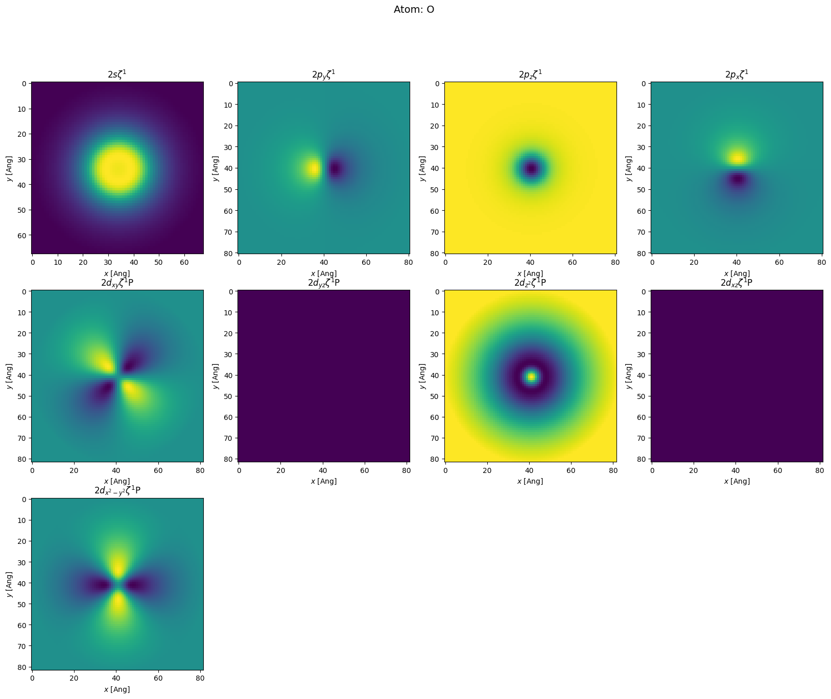
orthogonal: False. Secondly, we see it was an un-polarized calculation (Spin{unpolarized...).sisl. The oxygen has 9 orbitals (\(s+p+d\) where the \(d\) orbitals are \(p\)-polarizations denoted by capital P). We also see that it is a
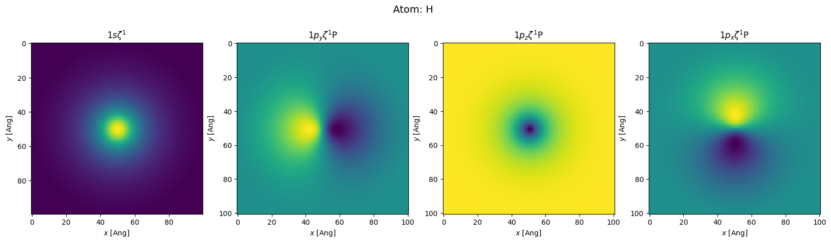
single-\(\zeta\) calculation Z1 (for double-\(\zeta\) Z2 would also appear in the list). The hydrogens only has 4 orbitals \(s+p\). For each orbital one can see its maximal radial part and how initial charges are distributed.Plotting orbitals
Often it may be educational (and fun) to plot the orbital wavefunctions. To do this we use the intrinsic method in the Orbital class named toGrid. The below code is rather complicated, but the complexity is simply because we want to show the orbitals in a rectangular grid of plots.
[7]:
def plot_atom(atom):
    no = len(atom)  # number of orbitals
    nx = no // 4
    ny = no // nx
    if nx * ny < no:
        nx += 1
    fig, axs = plt.subplots(nx, ny, figsize=(20, 5 * nx))
    fig.suptitle("Atom: {}".format(atom.symbol), fontsize=14)

    def my_plot(i, orb):
        grid = orb.toGrid(atom=atom)
        # In case you want to plot it with external software
        # Just uncomment the following line:
        # grid.write("{}_{}.cube".format(atom.symbol, orb.name()))
        c, r = i // 4, (i - 4) % 4
        if nx == 1:
            ax = axs[r]
        else:
            ax = axs[c][r]
        ax.imshow(grid.grid[:, :, grid.shape[2] // 2])
        ax.set_title(r"${}$".format(orb.name(True)))
        ax.set_xlabel(r"$x$ [Ang]")
        ax.set_ylabel(r"$y$ [Ang]")

    i = 0
    for orb in atom:
        my_plot(i, orb)
        i += 1
    if i < nx * ny:
        # This removes the empty plots
        for j in range(i, nx * ny):
            c, r = j // 4, (j - 4) % 4
            if nx == 1:
                ax = axs[r]
            else:
                ax = axs[c][r]
            fig.delaxes(ax)
        plt.draw()


plot_atom(h2o.atoms[0])
plot_atom(h2o.atoms[1])
Hamiltonian eigenstates
At this point we have the full Hamiltonian as well as the basis functions used in the Siesta calculation. This completes what is needed to calculate a great deal of physical quantities, e.g. eigenstates, density of states, projected density of states and wavefunctions.
To begin with we calculate the \(\Gamma\)-point eigenstates and plot a subset of the eigenstates’ norm on the geometry. An important aspect of the electronic structure handled by Siesta is that it is shifted to \(E_F=0\) meaning that the HOMO level is the smallest negative eigenvalue, while the LUMO is the smallest positive eigenvalue:
[8]:
es = H.eigenstate()

# We specify an origin to center the molecule in the grid
h2o.lattice.origin = [-4, -4, -4]

# Reduce the contained eigenstates to only the HOMO and LUMO
# Find the index of the smallest positive eigenvalue
idx_lumo = (es.eig > 0).nonzero()[0][0]
es = es.sub([idx_lumo - 1, idx_lumo])

plots = [
    h2o.plot(axes="xy", atoms_style={"size": normalize(n), "color": c})
    for n, c in zip(
        h2o.apply(
            es.norm2(projection="orbital"),
            np.sum,
            mapper=partial(h2o.a2o, all=True),
            axis=1,
        ),
        ("red", "blue", "green"),
    )
]

merge_plots(*plots, composite_method="subplots", cols=2)
These are not that interesting. The projection of the HOMO and LUMO states show where the largest weight of the HOMO and LUMO states, however we can’t see the orbital symmetry differences between the HOMO and LUMO states.
Instead of plotting the weight on each orbital it is more interesting to plot the actual wavefunctions which contains the orbital symmetries, however, matplotlib is currently not capable of plotting real-space iso-surface plots. To do this, please use VMD or your preferred software.
[9]:
def integrate(g):
    print(
        "Real space integrated wavefunction: {:.4f}".format(
            (np.absolute(g.grid) ** 2).sum() * g.dvolume
        )
    )


g = si.Grid(0.2, lattice=h2o.lattice)
es.sub(0).wavefunction(g)
integrate(g)
# g.write('HOMO.cube')
g.fill(0)  # reset the grid values to 0
es.sub(1).wavefunction(g)
integrate(g)
# g.write('LUMO.cube')
Real space integrated wavefunction: 1.0000
Real space integrated wavefunction: 1.0003
info:0: SislInfo:

wavefunction: coordinates may be outside your primary unit-cell. Translating all into the primary unit cell could disable this information

info:0: SislInfo:

wavefunction: coordinates may be outside your primary unit-cell. Translating all into the primary unit cell could disable this information
Real space charge
Since we have the basis functions we can also plot the charge in the grid. We can do this via either reading the density matrix or read in the charge output directly from Siesta. Since both should yield the same value we can compare the output from Siesta with that calculated in sisl.
You will notice that re-creating the density on a real space grid in sisl is much slower than creating the wavefunction. This is because we need orbital multiplications.
[10]:
DM = fdf.read_density_matrix()
rho = si.get_sile("siesta_1.nc").read_grid("Rho")
Create a new grid that is the negative of the readed charge density, then use sisl to calculate the charge density. This will check whether sisl and Siesta creates the same charge density.
[11]:
diff = rho * (-1)
DM.density(diff)
print(
    "Real space integrated density difference: {:.3e}".format(
        diff.grid.sum() * diff.dvolume
    )
)
Real space integrated density difference: -3.966e-04
[ ]: