GeometryPlot
[1]:
import sisl
import numpy as np
First of all, we will create a geometry to work with
[2]:
geom = sisl.geom.graphene_nanoribbon(9)
GeometryPlot allows you to quickly visualize a geometry. You can create a GeometryPlot out of a geometry very easily:
[3]:
# GeometryPlot is the default plot of a geometry, so one can just do
plot = geom.plot()
Now let’s see what we got:
[4]:
plot
_ipython_canary_method_should_not_exist_ False
_ipython_display_ True
Plotting in 3D, 2D and 1D
The 3D view is great, but for big geometries it can take some time to render. If we have a 2d material, a 2D view might be more practical instead. We can get it by specifying the axes that we want:
[5]:
plot.update_inputs(axes="xy")
_ipython_canary_method_should_not_exist_ False
_ipython_display_ True
The next section goes more in depth on what the axes setting accepts. The important part for now is that asking for two axes gets you a 2D representation. Samewise, asking for 1 axis gets you a 1D representation:
[6]:
plot.update_inputs(
axes="x",
)
_ipython_canary_method_should_not_exist_ False
_ipython_display_ True
Notice how asking for a 1D representation leaves the Y axis of the plot at your disposal. You can control the values in the second axis using the dataaxis_1d setting.
It can be an array that explicitly sets the values:
Or a function that accepts the projected coordinates and returns the values.
[7]:
plot.update_inputs(dataaxis_1d=np.sin)
_ipython_canary_method_should_not_exist_ False
_ipython_display_ True
Asking for three axes would bring us back to the 3D representation:
[8]:
plot.update_inputs(axes="xyz")
_ipython_canary_method_should_not_exist_ False
_ipython_display_ True
Specifying the axes
There are many ways in which you may want to display the coordinates of your geometry. The most common one is to display the cartesian coordinates. You indicate that you want cartesian coordinates by passing (+-){"x", "y", "z"}. You can pass them as a list:
[9]:
plot.update_inputs(axes=["x", "y"])
_ipython_canary_method_should_not_exist_ False
_ipython_display_ True
But it is usually more convenient to pass them as a multicharacter string:
[10]:
plot.update_inputs(axes="xy")
_ipython_canary_method_should_not_exist_ False
_ipython_display_ True
Notice that you can order axes in any way you want. The first one will go to the X axis of the plot, and the second to the Y axis:
[11]:
plot.update_inputs(axes="yx")
_ipython_canary_method_should_not_exist_ False
_ipython_display_ True
You are not limited to cartesian coordinates though. Passing (+-){"a", "b", "c"} will display the fractional coordinates:
[12]:
plot.update_inputs(axes="ab")
_ipython_canary_method_should_not_exist_ False
_ipython_display_ True
And you can also pass an arbitrary direction as an axis:
[13]:
plot.update_inputs(axes=[[1, 1, 0], [1, -1, 0]])
_ipython_canary_method_should_not_exist_ False
_ipython_display_ True
In this case, we have projected the coordinates into the [1,1,0] and [1, -1, 0] directions. Notice that the modulus of the vector is important for the scaling. See for example what happens when we scale the second vector by a factor of two:
[14]:
plot.update_inputs(axes=[[1, 1, 0], [2, -2, 0]])
_ipython_canary_method_should_not_exist_ False
_ipython_display_ True
Finally, you can even mix the different possibilities!
[15]:
plot.update_inputs(axes=["x", [1, 1, 0]])
_ipython_canary_method_should_not_exist_ False
_ipython_display_ True
To summarize the different possibilities:
(+-){"x", "y", "z"}: The cartesian coordinates are displayed.(+-){"a", "b", "c"}: The fractional coordinates are displayed. Same for {0,1,2}.np.array of shape (3, ): The coordinates are projected into that direction. If two directions are passed, the coordinates are not projected to each axis separately. The displayed coordinates are then the coefficients of the linear combination to get that point (or the projection of that point into the plane formed by the two axes).
Some non-obvious behavior
Fractional coordinates are only displayed if all axes are lattice vectors. Otherwise, the plot works as if you had passed the direction of the lattice vector. Also, for now, the 3D representation only displays cartesian coordinates.
2D perspective
It is not trivial to notice that the axes you choose determine what is your point of view. For example, if you choose to view "xy", the z axis will be pointing “outside of the screen”, while if you had chosen "yx" the z axis will point “inside the screen”. This affects the depth of the atoms, i.e. which atoms are on top and which are on the bottom.
To visualize it, we build a bilayer of graphene and boron nitride:
[16]:
bilayer = sisl.geom.bilayer(top_atoms="C", bottom_atoms=["B", "N"], stacking="AA")
If we want to see the "xy" axes, we would be viewing the structure from the top:
[17]:
bilayer.plot(axes="xy")
_ipython_canary_method_should_not_exist_ False
_ipython_display_ True
but if we set the axes to yx, -xy or x-y, we will see it from the bottom:
[18]:
bilayer.plot(axes="-xy")
_ipython_canary_method_should_not_exist_ False
_ipython_display_ True
That is, we are flipping the geometry. In the above example we are doing it around the Y axis. Notice that trying to view ``xy`` from the ``-z`` perspective would show you a mirrored view of your structure!
Non-cartesian axes
The above behavior is also true for all valid axes that you can pass. However, we have made lattice vectors follow the same rules as cartesian vectors. That is, abc cross products follow the rules of xyz cross products. As a result, if you ask for axes="ab" you will see the structure from the c perspective.
Toggling bonds, atoms and cell
You might have noticed that, by default, the cell, atoms and bonds are displayed. Thanks to plotly’s capabilities, you can interactively toggle them by clicking at the names in the legend, which is great!
However, if you want to make sure they are not displayed in the first place, you can set the show_bonds, show_cell and show_atoms settings to False.
[19]:
plot.update_inputs(axes="xy", show_cell=False, show_atoms=False)
_ipython_canary_method_should_not_exist_ False
_ipython_display_ True
Picking which atoms to display
The atoms setting of GeometryPlot allows you to pick which atoms to display. It accepts exactly the same possibilities as the atoms argument in Geometry’s methods.
Therefore, you can ask for certain indices:
[20]:
plot.update_inputs(atoms=[1, 2, 3, 4, 5], show_atoms=True, show_cell="axes")
# show_cell accepts "box", "axes" and False
_ipython_canary_method_should_not_exist_ False
_ipython_display_ True
or use sisl categories to filter the atoms, for example.
We can use it to display only those atoms that have 3 neighbours:
[21]:
plot.update_inputs(atoms={"neighbours": 3}, show_cell="box")
_ipython_canary_method_should_not_exist_ False
_ipython_display_ True
_ipython_canary_method_should_not_exist_ False
_repr_mimebundle_ True
_ipython_canary_method_should_not_exist_ False
_repr_html_ True
_ipython_canary_method_should_not_exist_ False
_repr_markdown_ False
_ipython_canary_method_should_not_exist_ False
_repr_svg_ False
_ipython_canary_method_should_not_exist_ False
_repr_png_ False
_ipython_canary_method_should_not_exist_ False
_repr_pdf_ False
_ipython_canary_method_should_not_exist_ False
_repr_jpeg_ False
_ipython_canary_method_should_not_exist_ False
_repr_latex_ False
_ipython_canary_method_should_not_exist_ False
_repr_json_ False
_ipython_canary_method_should_not_exist_ False
_repr_javascript_ False
[21]:
<sisl.viz.plots.geometry.GeometryPlot at 0x7fc4df7136e0>
Notice that when we picked particular atoms, only the bonds of those atoms are displayed. You can change this by using the bind_bonds_to_ats setting.
[22]:
plot.update_inputs(bind_bonds_to_ats=False)
_ipython_canary_method_should_not_exist_ False
_ipython_display_ True
_ipython_canary_method_should_not_exist_ False
_repr_mimebundle_ True
_ipython_canary_method_should_not_exist_ False
_repr_html_ True
_ipython_canary_method_should_not_exist_ False
_repr_markdown_ False
_ipython_canary_method_should_not_exist_ False
_repr_svg_ False
_ipython_canary_method_should_not_exist_ False
_repr_png_ False
_ipython_canary_method_should_not_exist_ False
_repr_pdf_ False
_ipython_canary_method_should_not_exist_ False
_repr_jpeg_ False
_ipython_canary_method_should_not_exist_ False
_repr_latex_ False
_ipython_canary_method_should_not_exist_ False
_repr_json_ False
_ipython_canary_method_should_not_exist_ False
_repr_javascript_ False
[22]:
<sisl.viz.plots.geometry.GeometryPlot at 0x7fc4df7136e0>
[23]:
plot = plot.update_inputs(atoms=None, bind_bonds_to_ats=True)
In fact, when we set show_atoms to False, all that the plot does is to act as if atoms=[] and bind_bonds_to_ats=False.
Scaling atoms
In the following section you can find extensive detail about styling atoms, but if you just one a quick rescaling of all atoms, atoms_scale is your best ally. It is very easy to use:
[24]:
plot.update_inputs(atoms_scale=0.6)
_ipython_canary_method_should_not_exist_ False
_ipython_display_ True
[25]:
plot.update_inputs(atoms_scale=1)
_ipython_canary_method_should_not_exist_ False
_ipython_display_ True
Custom styles for atoms.
It is quite common that you have an atom-resolved property that you want to display. With GeometryPlot this is extremely easy :)
All styles are controlled by the atoms_style setting. For example, if we want to color all atoms in green and with a size of 0.6 we can do it like this:
[26]:
plot.update_inputs(atoms=None, axes="yx", atoms_style={"color": "green", "size": 0.6})
_ipython_canary_method_should_not_exist_ False
_ipython_display_ True
In the following cell we show how these properties accept multiple values. In this case, we want to give different sizes to each atom. If the number of values passed is less than the number of atoms, the values are tiled:
[27]:
plot.update_inputs(atoms_style={"color": "green", "size": [0.6, 0.8]})
_ipython_canary_method_should_not_exist_ False
_ipython_display_ True
In this case, we have drawn atoms with alternating size of 0.6 and 0.8.
The best part about atoms_style is that you can very easily give different styles to selections of atoms. In this case, it is enough to pass a list of style specifications, including (optionally) the "atoms" key to select the atoms to which these styles will be applied:
[28]:
plot.update_inputs(
atoms_style=[
{"color": "green", "size": [0.6, 0.8], "opacity": [1, 0.3]},
{"atoms": [0, 1], "color": "orange"},
]
)
_ipython_canary_method_should_not_exist_ False
_ipython_display_ True
Notice these aspects:
The first specification doesn’t contain
"atoms", so it applies to all atoms.Properties that were not specified for atoms [0, 1] are “inherited” from the previous specifications. For example, size of atoms 0 and 1 is still determined by the first style specification.
If some atom is selected in more than one specification, the last one remains, that’s why the color is finally set to orange for
[0,1].
You don’t need to include general styles. For atoms that don’t have styles specified the defaults are used:
[29]:
plot.update_inputs(atoms_style=[{"atoms": [0, 1], "color": "orange"}])
_ipython_canary_method_should_not_exist_ False
_ipython_display_ True
Finally, "atoms" accepts anything that Geometry can sanitize, so it can accept categories, for example. This is great because it gives you a great power to easily control complex styling situations:
[30]:
plot.update_inputs(
atoms_style=[
{"atoms": {"fx": (None, 0.4)}, "color": "orange"},
{"atoms": sisl.geom.AtomOdd(), "opacity": 0.3},
]
)
_ipython_canary_method_should_not_exist_ False
_ipython_display_ True
In this case, we color all atoms whose fractional X coordinate is below 0.4 (half the ribbon) in orange. We also give some transparency to odd atoms.
As a final remark, colors can also be passed as values. In this case, they are mapped to colors by a colorscale, specified in atoms_colorscale.
[31]:
# Get the Y coordinates
y = plot.geometry.xyz[:, 1]
# And color atoms according to it
plot.update_inputs(
atoms_style=[
{"color": y},
{"atoms": sisl.geom.AtomOdd(), "opacity": 0.3},
],
atoms_colorscale="viridis",
)
_ipython_canary_method_should_not_exist_ False
_ipython_display_ True
Notice however that, for now, you can not mix values with strings and there is only one colorscale for all atoms.
Note that everything that we’ve done up to this moment is perfectly valid for the 3d view, we are just using the 2d view for convenience.
[32]:
plot.update_inputs(axes="xyz")
_ipython_canary_method_should_not_exist_ False
_ipython_display_ True
Custom styles for bonds
Just as atoms_style, there is a setting that allows you to tweak the styling of the bonds: bonds_style. Unlike atoms_style, for now only one style specification can be provided. That is, bonds_style only accepts a dictionary, not a list of dictionaries. The dictionary can contain the following keys: color, width and opacity, but you don’t need to provide all of them.
[33]:
plot.update_inputs(
axes="yx", bonds_style={"color": "orange", "width": 5, "opacity": 0.5}
).get()
As in the case of atoms, the styling attributes can also be lists:
[34]:
plot.update_inputs(
bonds_style={
"color": ["blue"] * 10 + ["orange"] * 19,
"width": np.linspace(3, 7, 29),
}
)
_ipython_canary_method_should_not_exist_ False
_ipython_display_ True
However, in this case, providing a list is more difficult than in the atoms case, because you don’t know beforehand how many bonds are going to be drawn (in this case 29) or which atoms will correspond to each bond.
For this reason, in this case it is much better to provide a callable that receives geometry and bonds and returns the property:
[35]:
def color_bonds(geometry: sisl.Geometry, bonds: "xr.DataArray"):
# We are going to color the bonds based on how far they go in the Y axis
return abs(geometry[bonds[:, 0], 1] - geometry[bonds[:, 1], 1])
plot.update_inputs(bonds_style={"color": color_bonds, "width": 5})
_ipython_canary_method_should_not_exist_ False
_ipython_display_ True
It is even better to use nodes, because they will not recompute the property if the styles need to be recomputed but the geometry and bonds haven’t changed.
In sisl.viz.data_sources you can find several Bond* nodes already prepared for you. BondLength is probably the most common to use, but in this case all bonds have the same length, so we are going to use BondRandom just for fun :)
[36]:
from sisl.viz.data_sources import BondLength, BondDataFromMatrix, BondRandom
plot.update_inputs(
axes="yx",
bonds_style={"color": BondRandom(), "width": BondRandom() * 10, "opacity": 0.5},
)
_ipython_canary_method_should_not_exist_ False
_ipython_display_ True
As with atoms, you can change the colorscale of the bonds with bonds_colorscale.
[37]:
plot.update_inputs(bonds_colorscale="viridis")
_ipython_canary_method_should_not_exist_ False
_ipython_display_ True
Bicolor bonds
Most rendering softwares display bonds with two colors, one for each half of the bond. This is not supported yet in sisl, but it is probably going to be supported in the future.
[38]:
plot = plot.update_inputs(axes="xyz", bonds_style={})
Drawing arrows
It is very common that you want to display arrows on the atoms, to show some vector property such as a force or an electric field.
This can be specified quite easily in sisl with the arrows setting. All the information of the arrows that you want to draw is passed as a dictionary, where "data" is the most important key and there are other optional keys like name, color, width, scale, arrowhead_scale and arrowhead_angle that control the aesthetics.
[39]:
plot.update_inputs(arrows={"data": [0, 0, 2], "name": "Upwards force"})
_ipython_canary_method_should_not_exist_ False
_ipython_display_ True
Notice how we only provided one vector and it was used for all our atoms. We can either do that or pass all the data. Let’s build a fake forces array for the sake of this example:
[40]:
forces = np.linspace([0, 0, 2], [0, 3, 1], 18)
plot.update_inputs(
arrows={"data": forces, "name": "Force", "color": "orange", "width": 4}
)
_ipython_canary_method_should_not_exist_ False
_ipython_display_ True
Since there might be more than one vector property to display, you can also pass a list of arrow specifications, and each one will be drawn separately.
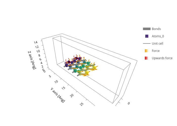
[41]:
plot.update_inputs(
arrows=[
{"data": forces, "name": "Force", "color": "orange", "width": 4},
{"data": [0, 0, 2], "name": "Upwards force", "color": "red"},
]
)
_ipython_canary_method_should_not_exist_ False
_ipython_display_ True
Much like we did in atoms_style, we can specify the atoms for which we want the arrow specification to take effect by using the "atoms" key.
[42]:
plot.update_inputs(
arrows=[
{"data": forces, "name": "Force", "color": "orange", "width": 4},
{
"atoms": {"fy": (0, 0.5)},
"data": [0, 0, 2],
"name": "Upwards force",
"color": "red",
},
]
)
_ipython_canary_method_should_not_exist_ False
_ipython_display_ True
Finally, notice that in 2D and 1D views, and for axes other than {"x", "y", "z"}, the arrows get projected just as the rest of the coordinates:
[43]:
plot.update_inputs(axes="yz")
_ipython_canary_method_should_not_exist_ False
_ipython_display_ True
Coloring individual atoms
It is still not possible to color arrows individually, e.g. using a colorscale. Future developments will probably work towards this goal.
Drawing supercells
All the functionality showcased in this notebook is compatible with displaying supercells. The number of supercells displayed in each direction is controlled by the nsc setting:
[44]:
plot.update_inputs(axes="xyz", nsc=[2, 1, 1]).show("png")
Notice however that you can’t specify different styles or arrows for the supercell atoms, they are just copied! Since what we are displaying here are supercells of a periodic system, this should make sense. If you want your supercells to have different specifications, tile the geometry before creating the plot.