.

WavefunctionPlot

The WavefunctionPlot class will help you very easily generate and display wavefunctions from a Hamiltonian or any other source. If you already have your wavefunction in a grid, you can use GridPlot.

Note

WavefunctionPlot is just an extension of GridPlot, so everything in the GridPlot notebook applies and this notebook will only display the additional features.

WavefunctionPlot changes the defaults of the axes and plot_geom inputs so that by default the grid is shown in 3D and displaying the geometry.

import sisl
import sisl.viz

Generating wavefunctions from a hamiltonian

We will create a toy graphene tight binding hamiltonian, but you could have read the Hamiltonian from any source. Note that your hamiltonian needs to contain the corresponding geometry with the right orbitals, otherwise we have no idea what’s the shape of the wavefunction.

import numpy as np

r = np.linspace(0, 3.5, 50)
f = np.exp(-r)

orb = sisl.AtomicOrbital("2pzZ", (r, f))
geom = sisl.geom.graphene(orthogonal=True, atoms=sisl.Atom(6, orb))
geom = geom.move([0, 0, 5])
H = sisl.Hamiltonian(geom)
H.construct(
    [(0.1, 1.44), (0, -2.7)],
)

Now that we have our hamiltonian, plotting a wavefunction is as simple as:

H.plot.wavefunction()

This is a very delocalized state, so its representation in 3D is not very interesting

Selecting the wavefunction

By default, WavefunctionPlot gives you the first wavefunction at the gamma point. You can control this behavior by tuning the i and k settings.

For example, to get the second wavefunction at the gamma point:

plot = H.plot.wavefunction(i=2, k=(0, 0, 0))
plot

You can also select the spin with the spin setting (if you have, of course, a spin polarized Hamiltonian).

Note

If you update the number of the wavefunction, the eigenstates are already calculated, so there’s no need to recalculate them. However, changing the k point or the spin component will trigger a recalculation of the eigenstates.

Grid precision

The wavefunction is projected in a grid, and how fine that grid is will determine the resolution. You can control this with the grid_prec setting, which accepts the grid precision in Angstrom. Let’s check the difference in 2D, where it will be best appreciated:

plot.update_inputs(axes="xy", transforms=["square"])  # by default grid_prec is 0.2 Ang

plot.update_inputs(grid_prec=0.05)

Much better, isn’t it? Notice how it didn’t look that bad in 3d, because the grid is smooth, so it’s values are nicely interpolated. You can also appreciate this by setting smooth to True in 2D, which does an “OK job” at guessing the values.

plot.update_inputs(grid_prec=0.2, smooth=True)

Warning

Keep in mind that a finer grid will occupy more memory and take more time to generate and render, and sometimes it might be unnecessary to make your grid very fine, specially if it’s smooth.

GridPlot settings

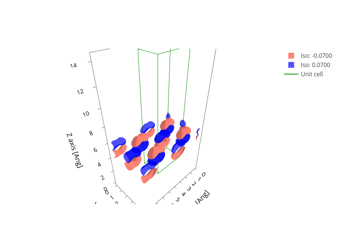
As stated at the beggining of this notebook, you have all the power of GridPlot available to you. Therefore you can, for example, display supercells of the resulting wavefunctions (please don’t tile the hamiltonian! :)).

plot.update_inputs(
    axes="xyz",
    nsc=[2, 2, 1],
    grid_prec=0.1,
    transforms=[],
    isos=[
        {"val": -0.07, "opacity": 1, "color": "salmon"},
        {"val": 0.07, "opacity": 0.7, "color": "blue"},
    ],
    geom_kwargs={"atoms_style": dict(color=["orange", "red", "green", "pink"])},
)

We hope you enjoyed what you learned!

---

This next cell is just to create the thumbnail for the notebook in the docs

thumbnail_plot = plot

if thumbnail_plot:
    thumbnail_plot.show("png")

---